

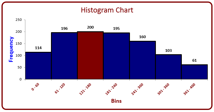
- Histogram charts are created by using BINS
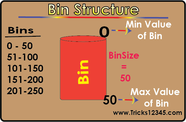
- We can define a particular range as BIN
- In the aforementioned instance 50 is the BIN size
- MIN value of the BIN is 0 and MAX value of the BIN is 50
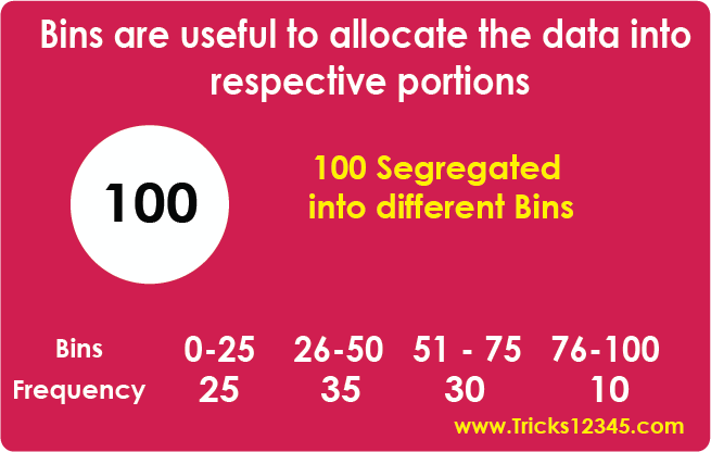
- Based above instance Total frequence allocated into respective bins depends on its sizes
Histogram Chart
What is Bin?
Click on below mentioned image to watch the video
Sub Create_Histogram_Chart_With_Dynamic_BinSize()
Application.DisplayAlerts = False
On Error Resume Next
ThisWorkbook.Sheets("Histogram Chart").Delete
Rem Create New worksheet to create Histogram chart at the end of sheets count
Dim SH As Worksheet
Set SH = ThisWorkbook.Sheets.Add(after:=ThisWorkbook.Sheets(Sheets.Count))
Rem Removing Gridlines in newly created worksheet
ActiveWindow.DisplayGridlines = False
Rem Storing Textbox values into Variables
MinValue = Val(UserForm1.TextBox1.Value)
MaxValue = Val(UserForm1.TextBox2.Value)
BinSize = Val(UserForm1.TextBox3.Value)
Unload UserForm1
ActualBinNumbers = (MaxValue - MinValue) / BinSize
Rem define Data Sheet
Dim DSH As Worksheet
Set DSH = ThisWorkbook.Sheets("Data Sheet")
Rem find Last Used cell row
LastRow = DSH.Range("A" & Rows.Count).End(xlUp).Row
Dim DataRange As Range
Set DataRange = DSH.Range("B1:B" & LastRow)
Rem Using For Loop to retrieve Bins & Count
For B = 1 To ActualBinNumbers
MinValueOfTheBin = MinValue
If B = 1 Then
MaxValueOfTheBin = MinValue + BinSize
Else: MaxValueOfTheBin = MinValue + BinSize - 1
End If
SH.Range("A" & 2 + B).Value = MinValueOfTheBin & " - " & MaxValueOfTheBin
SH.Range("B" & 2 + B).Value = _
Application.WorksheetFunction.CountIfs(DataRange, ">=" & MinValue, DataRange, "<=" & MaxValueOfTheBin)
MinValue = MaxValueOfTheBin + 1
Next
Rem If max value is not equal to Max value of the Bin
If MaxValueOfTheBin <> MaxValue Then
SH.Range("A" & 2 + B).Value = MaxValueOfTheBin + 1 & " - " & MaxValue
SH.Range("B" & 2 + B).Value = _
Application.WorksheetFunction.CountIfs(DataRange, ">=" & MaxValueOfTheBin + 1, DataRange, "<=" & MaxValue)
End If
SH.Range("A2").Value = "Bins"
SH.Range("B2").Value = "Frequency"
Rem Create Chart --- define chart object and its position in worksheet
Dim ch As ChartObject
With SH.Range("E3:O20")
Set ch = SH.ChartObjects.Add( _
Left:=.Left, _
Height:=.Height, _
Width:=.Width, _
Top:=.Top)
End With
With ch.Chart
.ChartType = xlColumnClustered
LastRow = SH.Range("A" & Rows.Count).End(xlUp).Row
.SetSourceData SH.Range("A2:B" & LastRow), PlotBy:=xlColumns
.SeriesCollection(1).Interior.ColorIndex = 25
.ChartArea.Border.ColorIndex = 30
.ChartArea.Border.Weight = xlThick
.ChartArea.RoundedCorners = True
.SetElement (msoElementPrimaryValueGridLinesNone)
.SetElement (msoElementPrimaryCategoryGridLinesNone)
Rem Find Max Value and highlight max value point with different color index
Dim FirstSeries As Series
Set FirstSeries = .SeriesCollection(1)
MaxValue = Application.WorksheetFunction.Max(SH.Range(Cells(3, 2), Cells(LastRow, 2)))
For P = 1 To FirstSeries.Points.Count
If FirstSeries.Values(P) = MaxValue Then
FirstSeries.Points(P).Interior.ColorIndex = 30
Exit For
End If
Next
Rem Formatting Series Axis
Dim SeriesAxis As Axis
Set SeriesAxis = .Axes(xlValue, xlPrimary)
SeriesAxis.HasTitle = True
SeriesAxis.AxisTitle.Caption = SH.Range("B2").Value
SeriesAxis.AxisTitle.Characters.Font.ColorIndex = 5
SeriesAxis.AxisTitle.Characters.Font.Size = 15
SeriesAxis.AxisTitle.Orientation = 90
SeriesAxis.HasMinorGridlines = False
SeriesAxis.HasMajorGridlines = False
Rem Formatting Category Axis
Dim XAxis As Axis
Set XAxis = .Axes(xlCategory)
XAxis.HasTitle = True
XAxis.AxisTitle.Caption = SH.Range("A2").Value
XAxis.AxisTitle.Characters.Font.ColorIndex = 30
XAxis.AxisTitle.Characters.Font.Size = 15
Rem Formatting TickLabels
Dim CategoryAxisTK As TickLabels
Set CategoryAxisTK = .Axes(xlCategory).TickLabels
CategoryAxisTK.Font.ColorIndex = 30
CategoryAxisTK.Orientation = 45
CategoryAxisTK.Font.Bold = True
Rem Formatting DataLabels
FirstSeries.HasDataLabels = True
Dim DataLble As DataLabels
Set DataLble = FirstSeries.DataLabels
DataLble.Font.Size = 11
DataLble.Font.Bold = True
DataLble.Font.Name = "Calibri"
DataLble.Orientation = xlHorizontal
Rem Formatting Chart Title
.HasTitle = True
Dim T As ChartTitle
Set T = .ChartTitle
T.Text = "Histogram Chart"
T.Font.ColorIndex = 30
T.Font.Size = 20
T.Font.FontStyle = "Century"
Rem Define the Postion of Legend
.HasLegend = False
'Dim L As Legend
'Set L = .Legend
'L.Position = xlLegendPositionTop
Rem Removing the Gaps between Points in SeriesCollection
With .ChartGroups(1)
.Overlap = 0
.GapWidth = 0
End With
Rem Providing Border Lines to series collection points
.FullSeriesCollection(1).Select
With Selection.Format.Line
.Weight = 2
.ForeColor.RGB = RGB(192, 0, 0)
.Visible = msoTrue
End With
End With
Rem Providing the sheet name
SH.Name = "Histogram Chart"
Application.DisplayAlerts = True
End Sub
Download The Workbook