

- Through this web automation we can retrieve company names from Yahoo web to excel workbook, by inserting symbols in search box.
- Click on image to view the video
- Import the data from Yahoo Finance
- Loop through all the elements of the IE Document and retrive the data when cell value mentioned in Header row having equivalent status with Inner text attribute of element
- After retrieving the data chart the values as per requirement, by selecting desired chart from combo box
- Update Index page by providing Hyperlinks to the sheet names
- Click on below extract to view the video
- This is the continuation to the aforementioned article
- Through this template user can import the provide the charting of data
- Yahoo Finance is providing the data to investors
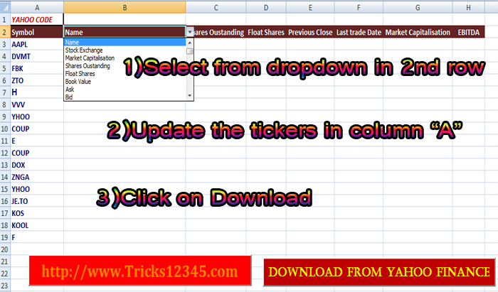
- We can download the data with the help of below mentioned template
- Select the DATA ITEMS in 2nd row from the available dropdown
- Update the tickers(for which company we want), in first column
- Click on COMMAND BUTTON to download in excel sheet
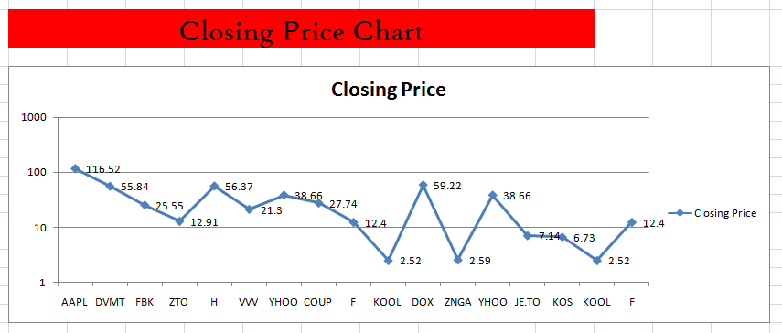
- This excel workbook consists of CHARTS for MARKET CAP, CLOSING PRICE,SHARES OUTSTANDING
- Click on respective COMMAND BUTTIONS to create CHARTS
Web Automation - Retrieve company Names - Ticker


Import Data and Charting techniques
Click on below image to view the video

Note: Below mentioned programs are not working
Web Automation - Import Market data from Yahoo

Web Automation:Import data from Yahoo and Charting

Download the data into excel from YAHOO
Steps to Follow:
Code:
Private Sub CommandButton1_Click()
Dim sh2 As Worksheet
Set sh2 = ThisWorkbook.Sheets("sheet2")
With sh2.Range("B2:H2").Validation
.Delete
.Add Type:=xlValidateList, AlertStyle:=xlValidAlertStop, Operator:=xlBetween, Formula1:="=Template_Features!A3:A47"
End With
'lookup function for field names
Dim code As String
Dim r As Integer
r = sh2.Range("B2").End(xlToRight).Column
For c = 2 To r
sh2.Cells(1, c) = Application.WorksheetFunction.VLookup(Cells(2, c), Sheets("Template_Features").Range("A3:B47"), 2, 0)
Columns(c).AutoFit
code = code & Cells(1, c).Value
Next
Dim max As Integer
Dim ticker
max = Range("A3").End(xlDown).Row
For i = 3 To max
ticker = sh2.Range("A" & i).Value
Dim url As String
url = "http://finance.yahoo.com/d/quotes.csv?s=" & ticker & "&f=" & code
Dim ht As New WinHttpRequest
ht.Open "get", url
ht.Send
Dim result
result = Split(ht.ResponseText, ",")
Dim parts As Integer, j As Integer
j = 2
For parts = 0 To UBound(result)
Cells(i, j).Value = result(parts)
Columns(j).AutoFit
j = j + 1
Next
UsedRange.WrapText = False
Next
End Sub
Create Chart
Download the Workbook
Create Chart for MARKET CAP
Sub marketcap()
On Error Resume Next
Application.DisplayAlerts = False
Sheets("Market Cap").Delete
Dim sh2 As Worksheet
Set sh2 = ThisWorkbook.Sheets("sheet2")
Dim max As Integer
max = sh2.Range("G3").End(xlDown).Row
Dim p As Integer
p = sh2.Range("A3").End(xlDown).Row
Dim sh As Worksheet
Set sh = Worksheets.Add(after:=Sheets("sheet2"))
sh.Name = "Market Cap"
Dim ch As ChartObject
With sh.Range("B4:K17")
Set ch = sh.ChartObjects.Add( _
Left:=.Left, _
Top:=.Top, _
Width:=.Width, _
Height:=.Height)
End With
sh2.Activate
Dim result As String
For i = 3 To max
j = Range("G" & i).Value
result = Left(j, Len(j) - 1)
sh.Range("O" & i).Value = result
sh.Range("N" & i).Value = sh2.Cells(i, 1).Value
Next
sh.Activate
With ch.Chart
'Define chart type
.ChartType = xlColumnClustered
'define max value of chart data
c = sh.Range("O3").End(xlDown).Row
.SetSourceData Source:=sh.Range("N3:O" & c), PlotBy:=xlColumns
.SeriesCollection(1).ApplyDataLabels
.SeriesCollection(1).Name = "Market Cap"
.Axes(xlValue).ScaleType = xlLogarithmic
End With
sh.Range("B2").Value = "Market Cap"
With sh.Range("B2:K2")
.HorizontalAlignment = xlCenterAcrossSelection
.Font.Size = 25
.Font.Name = "high tower text"
.Interior.ColorIndex = 3
End With
Application.DisplayAlerts = True
End Sub
Code:
Sub ClosingPrice()
On Error Resume Next
Application.DisplayAlerts = False
Sheets("Closing Price").Delete
Dim sh2 As Worksheet
Set sh2 = ThisWorkbook.Sheets("sheet2")
Dim max As Integer
max = sh2.Range("E3").End(xlDown).Row
Dim x As Integer
x = sh2.Range("A3").End(xlDown).Row
Dim sh As Worksheet
Set sh = Worksheets.Add(after:=Sheets("sheet2"))
sh.Name = "Closing Price"
Dim ch As ChartObject
With sh.Range("B4:N17")
Set ch = sh.ChartObjects.Add( _
Left:=.Left, _
Top:=.Top, _
Width:=.Width, _
Height:=.Height)
End With
With ch.Chart
.ChartType = xlLine
.SeriesCollection.NewSeries
.SeriesCollection(1).Name = "Closing Price"
.SeriesCollection(1).Values = sh2.Range("E3:E" & max)
.SeriesCollection(1).XValues = sh2.Range("A3:A" & x)
.SeriesCollection(1).ApplyDataLabels
.Axes(xlValue).ScaleType = xlLogarithmic
.SeriesCollection(1).Interior.Color = RGB(255, 0, 0)
End With
sh.Range("B2").Value = "Closing Price Chart"
With sh.Range("B2:K2")
.HorizontalAlignment = xlCenterAcrossSelection
.Font.Size = 25
.Font.Name = "high tower text"
.Interior.ColorIndex = 3
End With
Application.DisplayAlerts = True
End Sub
 Hi Everyone,
Welcome to VBA Macros Tutorial. This Tutorial provides comprehensive knowledge on VBA Macros to the user.
Hope it enhances your coding skills. If you like this web page kindly Share this to your near and dear.
I Prepared this content as per my level of knowledge, if any changes required kindly bring to my notice. Thanks for visiting this web page
Thanks,
Pavan Kumar Gundlapalli